PIDNet: Reading Notes
Overview
PIDNet is a real-time semantic segmentation network composed of three branches (P, I, and D) that work together to parse and preserve detailed information, aggregate context locally and globally, and extract high-frequency features to predict boundary regions.
There are different versions of PIDNet, such as PIDNet-L, PIDNet-M, and PIDNet-S, that differ in terms of their architecture and computational efficiency. Here I am using PIDNet-L as an example to explain the model structure.
Branch Structures
The PIDNet model uses the classic BasicBlock and Bottleneck to extract abstract semantic information. It consists of three branches: the Proportional (P) branch, the Integral (I) branch, and the Derivative (D) branch.
# filename="models/pidnet.py"

x = self.conv1(x)
x = self.layer1(x)
x = self.relu(self.layer2(self.relu(x)))

x_ = self.layer3_(x)
x_d = self.layer3_d(x)
x = self.relu(self.layer3(x))
Then it provides a 3-branch network, namely Proportional-Integral-Derivative Network (PIDNet), which is x_, x x_d for P, I, D branch seperately in the model script.
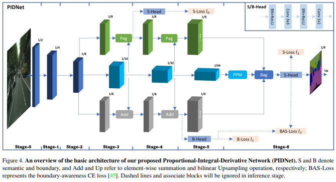
From the paper, PIDNet possesses three branches with complementary responsibilities: Proportional (P) branch parses and preserves the detailed information in its high-resolution feature maps; Integral (I) branch aggregates context information locally and globally to parse long-range dependencies; Derivative (D) branch extracts the high-frequency features to predict the boundary regions., which is shown on the following as Model Structure Overview
Proportional Branch
The P branch parses and preserves detailed information in its high-resolution feature maps, and generates moderate or detailed information to final result. The P branch is developed from the I branch, and is compressed using a Pag module.
Take the part from layer3 to layer4 as an example. It compresses information from P and the origin semantic branch I, using Pag (we would talk about it later) to generate the information of P branch on layer4.
# filename="models/pidnet.py"
# x_ is information from P branch and x is from I branch

self.compression3 = nn.Sequential(
                                nn.Conv2d(planes * 4, planes * 2, kernel_size=1, bias=False),
                                BatchNorm2d(planes * 2, momentum=bn_mom),
                                )
self.pag3 = PagFM(planes * 2, planes)

x_ = self.pag3(x_, self.compression3(x))
Generally, P branch provides the moderate, or detailed information, and at the last step, it can help I branch to produce result using Bag module (we could talk about it in the next part)
Integral Branch
The I branch aggregates context information locally and globally to parse long-range dependencies. It is designed to provide backup information to the P and D branches, and is crucial for the detail parsing of the P branch. The I branch provides one part of the final output by multiplying the weight generated from the D result.
This is code from layer3 to layer 4 in Integral Branch
# filename="models/pidnet.py"
# x is information from I branch

self.layer4 = self._make_layer(BasicBlock, planes * 4, planes * 8, n, stride=2)
x = self.relu(self.layer4(x))
At the final stage, it would contribute one part of final output by multipling weight generated from D result. It can be written in code as:
# filename="models/pidnet.py"

edge_att = torch.sigmoid(d)
return self.conv(edge_att*p + (1-edge_att)*i)
Derivative Branch
The D branch extracts high-frequency features to predict boundary regions and control the output before overshoot happens. It helps improve the model’s performance on edge prediction by coping with overshooting issues on object edges. In other words, with its help, we can improve model performance on edge prediction.
Take an example on getting information of layer3 on D Branch from layer3 on I branch here.
# filename="models/pidnet.py"
# x_d is result from d branch

self.diff3 = nn.Sequential(
                        nn.Conv2d(planes * 4, planes, kernel_size=3, padding=1, bias=False),
                        BatchNorm2d(planes, momentum=bn_mom),
                        )
x_d = x_d + F.interpolate(
                self.diff3(x),
                size=[height_output, width_output],
                mode='bilinear', align_corners=algc)
On the final layer, it would works as weight for branch P and I, in math, weight * x + (1-weight) * x_ (x is information from P and x_ is from I)
PAPPM
PAPPM (Parallel Aggregation PPM) is a context harvesting module designed to improve the global scene understanding in computer vision models. It operates similarly to Spatial Pyramid Pooling (SPP) in SwiftNet, by aggregating information at multiple scales to capture global dependencies and enhance the model’s predictions.
While PIDNet-M and PIDNet-S use PAPPM to speed up the context aggregation process, the author of PIDNet-L decided to stick with DAPPM due to its deeper architecture.
PAPPM operates by using a Pyramid CNN to process the input feature maps at multiple scales, followed by a channel reduction operation to reduce the dimensionality of the feature maps. The resulting feature maps are then rescaled back to their original sizes and concatenated with the input feature maps to form the final output. Unlike other context harvesting modules, PAPPM performs parallel aggregation of information at different scales, which reduces the computational cost and improves the model’s speed while maintaining high accuracy.
By aggregating information at multiple scales, PAPPM enables the model to capture both fine-grained and coarse-grained details, and enhances its ability to perform global scene understanding. 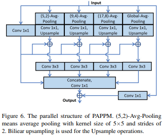
models/model_utils.py
# filename="models/model_utils.py"

class PAPPM(nn.Module):
    def __init__(self, inplanes, branch_planes, outplanes, BatchNorm=nn.BatchNorm2d):
        super(PAPPM, self).__init__()
        bn_mom = 0.1
        self.scale1 = nn.Sequential(nn.AvgPool2d(kernel_size=5, stride=2, padding=2),
                                    BatchNorm(inplanes, momentum=bn_mom),
                                    nn.ReLU(inplace=True),
                                    nn.Conv2d(inplanes, branch_planes, kernel_size=1, bias=False),
                                    )
        self.scale2 = nn.Sequential(nn.AvgPool2d(kernel_size=9, stride=4, padding=4),
                                    BatchNorm(inplanes, momentum=bn_mom),
                                    nn.ReLU(inplace=True),
                                    nn.Conv2d(inplanes, branch_planes, kernel_size=1, bias=False),
                                    )
        self.scale3 = nn.Sequential(nn.AvgPool2d(kernel_size=17, stride=8, padding=8),
                                    BatchNorm(inplanes, momentum=bn_mom),
                                    nn.ReLU(inplace=True),
                                    nn.Conv2d(inplanes, branch_planes, kernel_size=1, bias=False),
                                                                        )
        self.scale4 = nn.Sequential(nn.AdaptiveAvgPool2d((1, 1)),
                                    BatchNorm(inplanes, momentum=bn_mom),
                                    nn.ReLU(inplace=True),
                                    nn.Conv2d(inplanes, branch_planes, kernel_size=1, bias=False),
                                    )

        self.scale0 = nn.Sequential(
                                    BatchNorm(inplanes, momentum=bn_mom),
                                    nn.ReLU(inplace=True),
                                    nn.Conv2d(inplanes, branch_planes, kernel_size=1, bias=False),
                                    )

        self.scale_process = nn.Sequential(
                                    BatchNorm(branch_planes*4, momentum=bn_mom),
                                    nn.ReLU(inplace=True),
                                    nn.Conv2d(branch_planes*4, branch_planes*4, kernel_size=3, padding=1, groups=4, bias=False),
                                    )


        self.compression = nn.Sequential(
                                    BatchNorm(branch_planes * 5, momentum=bn_mom),
                                    nn.ReLU(inplace=True),
                                    nn.Conv2d(branch_planes * 5, outplanes, kernel_size=1, bias=False),
                                    )

        self.shortcut = nn.Sequential(
                                    BatchNorm(inplanes, momentum=bn_mom),
                                    nn.ReLU(inplace=True),
                                    nn.Conv2d(inplanes, outplanes, kernel_size=1, bias=False),
                                    )


    def forward(self, x):
        width = x.shape[-1]
        height = x.shape[-2]
        scale_list = []
        x_ = self.scale0(x)
        scale_list.append(F.interpolate(self.scale1(x), size=[height, width],
                        mode='bilinear', align_corners=algc)+x_)
        scale_list.append(F.interpolate(self.scale2(x), size=[height, width],
                        mode='bilinear', align_corners=algc)+x_)
        scale_list.append(F.interpolate(self.scale3(x), size=[height, width],
                        mode='bilinear', align_corners=algc)+x_)
        scale_list.append(F.interpolate(self.scale4(x), size=[height, width],
                        mode='bilinear', align_corners=algc)+x_)

        scale_out = self.scale_process(torch.cat(scale_list, 1))

        out = self.compression(torch.cat([x_,scale_out], 1)) + self.shortcut(x)
        return out
Connection: Pag
To generate results in the P branch, information from the last layer of both P and I branches is combined. However, instead of using simple methods such as addition or multiplication, the author introduces a new node called Pag. In mathematical terms, this can be expressed as: σ = Sigmoid(fp(v~p)· fi(~vi)). In paper, the author compares the performance of different methods, including the Pag node and the Bag node (used for the final layer, which will be discussed later). The results show that using the Pag (and Bag) nodes can improve model performance by approximately 1%. The Pag node is a combination of CNN, BatchNorm, and ReLU layers, and its structure is shown in the accompanying image.
It’s important to note that the Pag node is just one of several improvements introduced in the paper to enhance model performance. Other modifications, such as the Parallel Aggregation PPM (PAPPM) module, are also crucial for improving the speed and accuracy of the PIDNet model. models/model_utils.py
# filename="models/model_utils.py"

class PagFM(nn.Module):
    # a = PagFM(planes * 2, planes)
    # a(x = (2*plane, 128, 128), y =(2*plane, 64, 64))

    def __init__(self, in_channels, mid_channels, after_relu=False, \
                with_channel=False, BatchNorm=nn.BatchNorm2d):
        super(PagFM, self).__init__()
        self.with_channel = with_channel
        self.after_relu = after_relu
        self.f_x = nn.Sequential(
                                nn.Conv2d(in_channels, mid_channels,
                                          kernel_size=1, bias=False),
                                BatchNorm(mid_channels)
                                )
        self.f_y = nn.Sequential(
                                nn.Conv2d(in_channels, mid_channels,
                                          kernel_size=1, bias=False),
                                BatchNorm(mid_channels)
                                )
        if with_channel:
            self.up = nn.Sequential(
                                    nn.Conv2d(mid_channels, in_channels,
                                              kernel_size=1, bias=False),
                                    BatchNorm(in_channels)
                                   )
        if after_relu:
            self.relu = nn.ReLU(inplace=True)

    def forward(self, x, y):
        input_size = x.size()
        if self.after_relu:
            y = self.relu(y)
            x = self.relu(x)

        y_q = self.f_y(y)
        y_q = F.interpolate(y_q, size=[input_size[2], input_size[3]],
                            mode='bilinear', align_corners=False)
        x_k = self.f_x(x)

        if self.with_channel:
            sim_map = torch.sigmoid(self.up(x_k * y_q))
        else:
            sim_map = torch.sigmoid(torch.sum(x_k * y_q, dim=1).unsqueeze(1))

        y = F.interpolate(y, size=[input_size[2], input_size[3]],
                            mode='bilinear', align_corners=False)
        x = (1-sim_map)*x + sim_map*y

        return x
Connection: Bag
The Boundary-Attention-Guided Fusion Module (BAG) is a powerful tool for combining the features provided by all three branches of our network. While the I branch is highly semantic and can offer precise semantics, it often loses important spatial and geometric details, particularly in the boundary region and for small objects.
However, thanks to the detailed P branch, which preserves spatial details better, the model can be trained to trust the detailed branch more in the boundary region and to use the context features to fill in the area inside objects.
By using a boundary attention mechanism, BAG is able to selectively emphasize the P branch features along the boundaries while still leveraging the semantic information provided by the I branch
This approach leads to more accurate and robust results, especially when dealing with complex scenes with intricate objects and boundaries.
# filename="models/model_utils.py"

class Light_Bag(nn.Module):
    def __init__(self, in_channels, out_channels, BatchNorm=nn.BatchNorm2d):
        super(Light_Bag, self).__init__()
        self.conv_p = nn.Sequential(
                                nn.Conv2d(in_channels, out_channels,
                                          kernel_size=1, bias=False),
                                BatchNorm(out_channels)
                                )
        self.conv_i = nn.Sequential(
                                nn.Conv2d(in_channels, out_channels,
                                          kernel_size=1, bias=False),
                                BatchNorm(out_channels)
                                )

    def forward(self, p, i, d):
        edge_att = torch.sigmoid(d)

        p_add = self.conv_p((1-edge_att)*i + p)
        i_add = self.conv_i(i + edge_att*p)

        return p_add + i_add
Loss Function
This structure use loss generated from P, I and D branch. For semantic loss, one is from P branch, shown as S-Loss l0 in Model Structure Overview . How to get it? The prediction is the result compared between interpolation of the layer3 on P branch and ground truth.
For S-Loss l1, the pred is from the final result from I branch, as it shows on Model Structure Overview. In the code, we can see, the author write it as class OhemCrossEntropy. For the forward, it has two parts.
- One part is
_ohem_forward(selecting the pred pobability less than the threshold, instead of calculating all pred probability loss), which uses the OHEM (Online Hard Example Mining) algorithm to select the hard samples and assign higher weights to their losses. This can help the network to focus on the difficult samples and improve the overall performance. - The other part is
_ce_forwardwhose roots is equal toCrossEntropyLoss. - The weight from
ohem_forwardand_ce_forwardis adjustable based on training
For boundary loss, it has two sources. One is the result from layer4 on D branch, the author used binary_cross_entropy_with_logits to build BoundaryLoss class with comparision to binary ground truth (have label as 1 else 0).
And the other result in boundary loss is from I branch. However, its ground truth is filtered as torch.where(torch.sigmoid(outputs[-1][:,0,:,:])>0.7, batch_labels, filler), which represents, the ground truth boundary is whose pixel confidence of output is pretty high (default is > 0.7), then use ohem_formward from class OhemCrossEntropy to combine the loss.
Finally we gonna get the mean of 4 types of loss to go backward to update the model paramters.
Creation
- Model structure: To alleviate this dual-branch problem, the author propose a novel three-branch network architecture: PIDNet, which is able to parse detail, context and boundary information (semantic derivatives), respectively, and adopts boundary attention to guide the attention of details and context.
In the dual-branch network architecture, the direct fusion of low-level details and high-level semantics will lead to the phenomenon that detailed features are easily overwhelmed by surrounding context information – overshooting, which limits the improvement of the accuracy of existing dual-branch models.
For combining results from the three branches, the author proposed using either the Boundary-attention-guided fusion (Bag) module or the Parallel Aggregation PPM (PAPPM) module. We will evaluate the performance of both modules and select the one that yields the best results.
- To calculate the loss, the author updated the ground truth based on the output of the branches, by using different layers of each branch to calculate the loss, as different layers capture different levels of detail and context. Additionally, use the
OhemCrossEntropyto calculate the semantic loss, which selects predicted probabilities less than a threshold for efficient training. Finally, calculate the mean of the four types of loss to update the model parameters.
Interesting part is, how does the author experiment with different layer combinations and select the one (layer3 on P branch and layer 4 on I branch) that yields the best results?
Training
To define the constant values for training, the author provides a *.yaml file. While this is a widely-used method, it is also recommended to write a *.yaml file for every training session to ensure consistency and reproducibility during daily fun time.
The training code provided finalizes the training and validation functions in utils/functions.py. While this makes the main script easy to follow, it may be difficult to troubleshoot errors that occur during training or validation.
It is important to note when to save the model during training. The author provides three different files: best.pt to store the best model based on validation results, checkpoint.pth.tar to save the current state including the model weights, optimizer state, best mIOU, and epoch, which can be used to resume training, and final_state.pt to store the final state of the model after training is completed. If the model cannot be updated after several epochs, final_state.pt can be used for testing and hyperparameter tuning.
Evaluation
The evaluation process is focused on calculating the confusion matrix and using it to calculate metrics such as accuracy, mIOU, and precision. For obstacle segmentation, the TP_rate (TP / Pos) is a key metric as it represents the number of correctly predicted pixels among the ground truth.
Firstly, for the confusion matrix, it uses seg_gt * num_class + seg_pred as index, and np.bicount to calculate the number of value per index, which can be written as following:
index = (seg_gt * num_class + seg_pred).astype('int32')
confusion_matrix = np.zeros((num_class, num_class))

for i_label in range(num_class):
    for i_pred in range(num_class):
        cur_index = i_label * num_class + i_pred
        if cur_index < len(label_count):
            confusion_matrix[
                    i_label,
                    i_pred
            ] = label_count[cur_index]
Then the confusion matrix can be formed as the following,
- Assumption: class 1 is TP
Column is for Ground Truth and row for Prediction
| Ground Truth/Prediction | 0 | 1 |
|---|---|---|
| 0 | TP | FN |
| 1 | FP | TP |
- Based on this confusion matrix, we can calculate the paramters using the following code:
confusion_matrix.py
# cm_t is confusion matrix
def calculation_from_confusion_matrix(
    cm, ignore_index = 0, return_iou_only=False
):
    #  ___ pre
    # |
    # |
    # gt

    cm_t = cm.compute()
    if ignore_index == 0:
        cm_t = cm_t[1:, 1:]

    res = torch.sum(cm_t, 0)  # for every class on gt
    pos = torch.sum(cm_t, 1)  # for every class on pre
    TP = torch.diagonal(cm_t)
    FN = torch.sum(cm_t, 1) - TP
    FP = torch.sum(cm_t, 0) - TP
    TN = torch.sum(cm_t) - (FP + FN + TP)

    # ACC
    PIXEL_ACC = torch.sum(TP) / torch.sum(pos)

    AVG_ACC = torch.nanmean(torch.where(pos>0, TP/pos, torch.nan))  # TP/np.maximum(1.0, pos) same as TPR
    all = pos + res - TP
    IOU_ARRAY = torch.where(all > 0, TP/all, torch.nan)

    AVG_IOU = torch.nanmean(IOU_ARRAY)

    if return_iou_only:
        return AVG_IOU, IOU_ARRAY

    # Sensitivity, hit rate, recall, or true positive rate  # what we care for auto driving
    TPR = torch.where((TP + FN) > 0, TP/(TP + FN), torch.nan)

    # Specificity or true negative rate
    TNR = torch.where((TN + FP) > 0, TN/(TP + FN), torch.nan)

    # Precision or positive predictive value
    PPV = torch.where((TP + FP) > 0,  TP/(TP + FN), torch.nan)

    # Negative predictive value
    NPV = torch.where((TN + FN) > 0, TN/(TN + FN), torch.nan)

    # Fall out or false positive rate
    FPR = torch.where((FP + TN) > 0, FP/(TN + FP), torch.nan)

    # False negative rate
    FNR = torch.where((TP + FN) > 0,  FN/(TP + FN), torch.nan)

    # False discovery rate
    FDR = torch.where((TP + FP) > 0, FP/(TP + FP), torch.nan)

    class_len = len(TPR)

    AVG_TPR = torch.nanmean(TPR)
    AVG_TNR = torch.nanmean(TNR)
    AVG_PPV = torch.nanmean(PPV)
    AVG_NPV = torch.nanmean(NPV)
    AVG_FPR = torch.nanmean(FPR)
    AVG_FNR = torch.nanmean(FNR)
    AVG_FDR = torch.nanmean(FDR)

    metrices = {
        "TPR": TPR,
        "TNR": TNR,
        "PPV": PPV,
        "NPV": NPV,
        "FPR": FPR,
        "FNR": FNR,
        "FDR": FDR,
        "PIXEL_ACC": PIXEL_ACC,
        "IOU_ARRAY": IOU_ARRAY,
        "AVG_TPR": AVG_TPR,
        "AVG_TNR": AVG_TNR,
        "AVG_PPV": AVG_PPV,
        "AVG_NPV": AVG_NPV,
        "AVG_FPR": AVG_FPR,
        "AVG_FNR": AVG_FNR,
        "AVG_FDR": AVG_FDR,
        "AVG_ACC": AVG_ACC,
        "AVG_IOU": AVG_IOU,
    }
    return metrices, cm_t
This is my current understanding. Please feel free to ask any question or provide any comment to help improve upon it!